SKILLS REQUIRED
ANSYS Fluent
Fluid Dynamics
Turbulent Flow
Pipe Analysis
SUMMARY: Collection of Computational Fluid Dynamics (CFD) projects

CFD is used to predict behavior of fluids in MANY different enviornments
DESCRIPTION:
This course was unusual in that the course consisted solely of projects that needed to be completed. The main reason: students already knew the Fluid Dynamics theory from several previous courses. The purpose of these projects was to learn how to input the theory into a computer and predict the resulting motion. I used ANSYS Fluent as the dedicated CFD package because of its higher fidelity and its ability to predict flow - a notoriously difficult task considering the equations of motion for fluids has not been solved completely analytically despite centuries of study.
Before proceeding, several concepts need to be introduced to help when explaining these projects:
Laminar vs. Turbulent Flow: Laminar Flow is when fluids are moving in “calm/orderly” fashion - contrasted against Turbulent FLow which is highly “chaotic” and difficult to track individual particles in the flow
Reynold’s Number (Re): Reynold’s Number is essentially an indicator for how Laminar (calm) or Turbulent (chaotic) a flow is. Lower values of Reynold’s Number correspond to Laminar Flow. The transition between Laminar Flow and Turbulent flow starts around 2500 < Re < 3500
Steady vs. Unsteady Flow: Steady Flow is when the rate of fluid flow does not change over time whereas Unsteady Flow occurs when the flow-rate changes over time. Using a faucet as an example comparison: Unsteady Flow occurs when the faucet is being turned on to its max setting vs. Steady Flow occurs when the faucet has already been turned on to its max flow setting.
Boundary layer separation: An event where a flow previously attached to an object detaches from said object. It should be noted that separation of flow DOES NOT mean that no flow occurs there (flow can come back later as an area called a “Zone of Recirculation”). An example of boundary layer separation would be if stall on an airplane occurs - an event where too much of the fluid (air) has detached from the surface of the airplane wing.

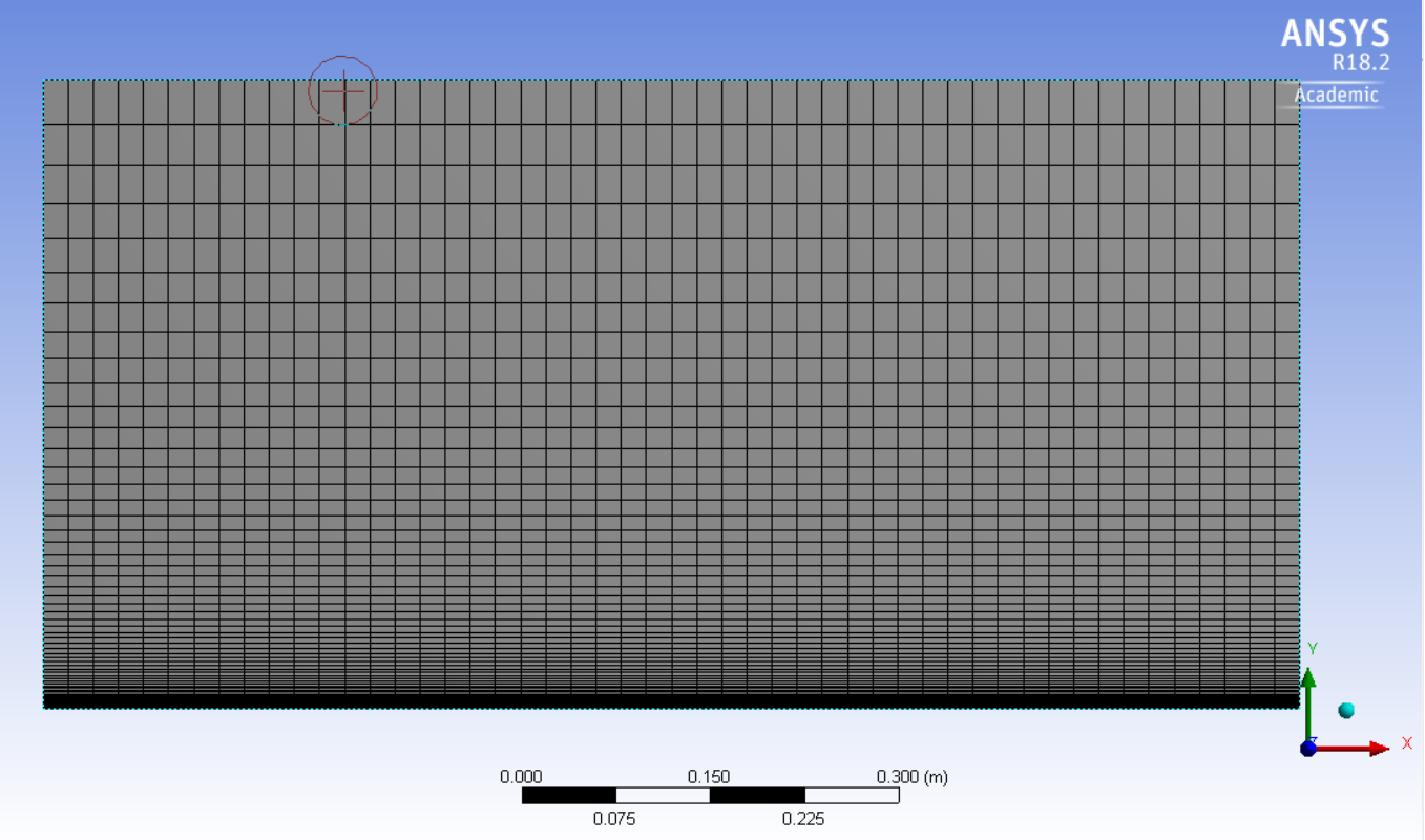
Meshing is when you subdivide a geometry into tiny shapes where you can make calculations on those tiny shapes to APPROXIMATE a physical scenario
To analyze the different scenarios, the subsequent steps were followed for ALL studies:
Step 1: Create geometry either in the program itself or imported geometry from SolidWorks
Step 2: Break up the geometry into a “mesh”
Step 3: Set the boundary conditions (geometric and fluidic)
Step 4: Set the flow conditions at inlet and outlet
Step 5: Specify how many particles (called “elements”) are desired in the simulation, which determines how the different flow properties are traced.
The previous steps are necessary to do the simulations themselves; procedurally, however, I take additional steps to set up the analytical solutions against which the numerical solutions (simulations) are compared against. Finally, the last topic that should be discussed before talking about the projects themselves are the “residuals”, which are errors that occur between iterations. Simulations work by running elements thousands of times; if the number of residuals (errors) goes towards zero, you have a simulation that works as intended and the equations agree with the results. If the residuals increase from iteration to iteration, there’s a problem in the simulation and the equations are not agreeing with the results.
Laminar Flow (left) can be described as “Orderly” or “Calm” while Turbulent Flow (right) can be described as “Rough” or “Chaotic”
With the basics out of the way, I start with the first study, which was how I created a simulation of a Laminar Flow over a Flat Plate. This scenario is a decent approximation of flow in the center of long pipes or corridors after flow has “Fully Developed” (i.e. the cross-sectional velocity no longer changes). The Laminar Flow over a Flat Plate case is also the main building block for more complicated simulations. The main takeaways for this study - and subsequent simulations - is the simulation will have different results than what theory prescribes. The consequences of this finding are two -fold: the first lesson learned is that simulations can act as a foil against analytical derivations of systems. The second lesson learned is that CFD can be treated as an “Experiment” in of itself as an additional means to validate test results and real-world phenomena. From a fluids perspective, the main takeaway is that the simulation was able to corroborate the phenomena that the boundary layer grows as the fluid flows over the plate (the friction between the fluid and the plate causes parts of the fluid to slow down; this region is called the “boundary layer”, which itself can be either Laminar or Turbulent).

The next study covered is laminar flow in an axisymmetric pipe. Since pipes are the building blocks of many fluid systems and laminar flows are the easiest to analyze, understanding how laminar flows in a pipe is essential to knowing how fluids behave. The main purpose of this simulation was to study how different mesh sizes affect the simulation results. For the flow characteristics, they behave similarly to the flat plate case in that the boundary layer increases and the skin friction coefficient decreases as you get further away from the starting point (inlet); additionally, because a long pipe was used, there comes a point where the flow becomes Fully Developed.
The results also confirmed observations that the cross-sectional velocity profile has a smoother “arch” when the flow is fully developed. When it comes to the effect different mesh sizes have on the simulation, the finer the mesh you have the longer the simulation takes and the numerical solutions approach the analytical solution as the mesh becomes finer. These results hold so long as the different simulation flow characteristics’ solutions converge (i.e. the residuals go towards zero) and the scenario has a definitive analytical solution.
After the Laminar flow in a Pipe was the exact same study except Turbulent Flow instead of Laminar. Because turbulence can be experimentally verified only as of present (ie. some components of the analytical solutions are inherently unknowable), scientists and engineers have to use approximate models that try to predict turbulent behavior. The specific turbulence model I used is called the k-Epsilon model, of which the most important point is that it is the simplest way to model turbulent flow with acceptable errors/results. The main findings from the overall Turbulent Flow in a Pipe study include:
Study confirms observations that as inlet velocity increases, distance for flow to become fully developed also increases
Study confirms observations that as Re increases, the skin coefficient increases more slowly than laminar flows because turbulence dissipates energy in the area.

Difference between Laminar Boundary Layer vs. Turbulent Boundary Layer
The next study deals with a steady, laminar flow ACROSS a pipe. These types of flows are routinely spotted in different engineering scenarios and are considered a fundamental analogy to many flows. A fitting analogy for this situation is the flow over an airplane wing during LOW speed operation.
The key takeaway from this simulation is that as the flow goes around the cylinder, the results from the simulation reaffirm the physical phenomena that flow separates from the cylinder at a certain point. However, a portion of the flow comes back to that region via a “Zone of Recirculation” with the location of flow separation measured as an angle relative to the center of the cylinder and the inlet of the bulk flow. This angle is called the “separation angle” and was found to increase (relative to the inlet) as Re increases, which is in line with real-world experiments.


The next project is the same as the previous study except that the flow varies with time. In other words, the simulation is a study of a Laminar, UNSTEADY Flow over a cylinder. The same findings apply as the previous study except there is a new phenomenon at play: vortex shedding. To briefly summarize what vortex shedding is, vortex shedding occurs when vortices form off a body (like a cylinder) and the vortices detach in an oscillating manner away from the body.
Vortex shedding has some very important effects on the fluid’s flow and affects the lift coefficient, drag coefficient, pressure coefficient, skin friction coefficient, and separation angle. The previous stated characteristics are affected by vortex shedding and affirms physical observations as follows:
Lift Coefficient: oscillates and grows with time until the lift coefficient reaches its stable oscillation
Drag Coefficient: Same effect as Lift Coefficient
Skin Friction Coefficient and Separation Angle: separation occurs (by definition) when C_f=0, which occurs when 105° < theta < 115°
Pressure Coefficient: Pressure of fluid starts resisting flow direction and occurs after C_p=0 on the front half of the cylinder (between 30° < theta < 35° for tested Re and meshes)

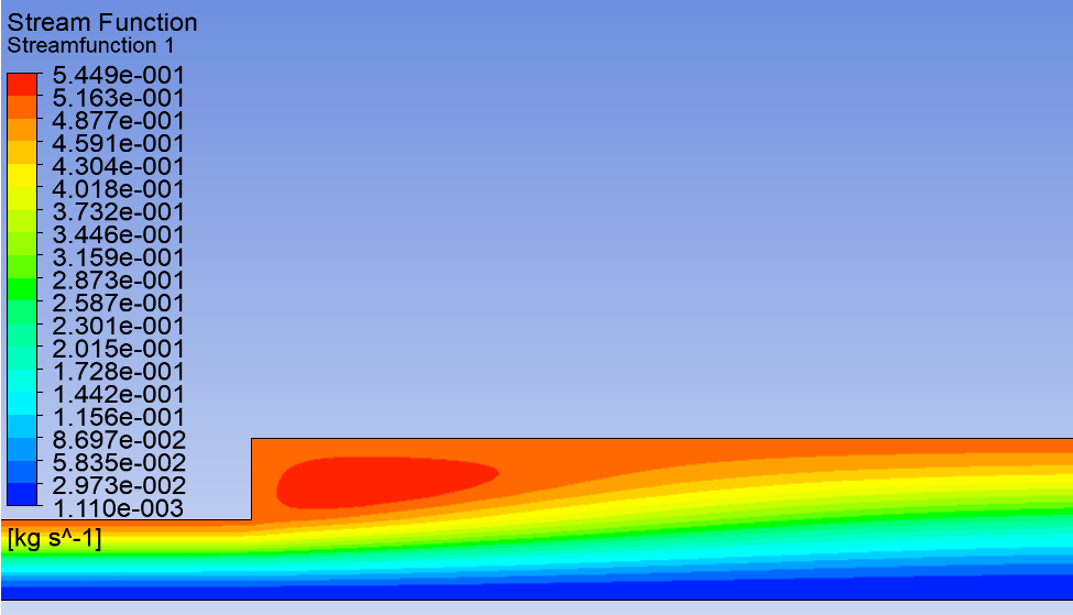
The idea of steady, laminar pipe flow is reexamined in this next study but with the addition of a slightly different geometry - a pipe with a sudden change in diameter. An example of where this different geometry occurs is when two pipes of different diameter suddenly join. This simulation focuses on the situation of going from a smaller diameter pipe to a larger one - termed a “Sudden Expansion”. Because fluids cannot flow at 90°, this creates a Recirculation Zone that greatly increases the drag of the fluid in a system. Because this recirculation zone creates a sizable increase in drag in the system and because this situation is common in the real world, it is a key situation to understand. The key takeaways from this study include:
As Re increases, the magnitude of the Eddy Strength (a ratio that shows how much fluid is flowing in the recirculation zone) increases
As Re increases, the center of the Eddy moves further away from the Sudden Expansion
As Re increases, the reattachment length (a measure of how big the recirculation zone is) also increases

Y-Plus - a measure how the height of the boundary layer for a turbulent flow - proved to have widely different results for different meshes and did not converge to an answer
The last study performed is the same as the previous study except instead of the flow being laminar, the flow is turbulent. The same findings apply to the Turbulent Flow w/ a Sudden Expansion as the Laminar Flow w/ a Sudden Expansion with some modifications. Again, the k-epsilon model is used to approximate turbulent flow. As such, the model produces similar results across different meshes in the direction of bulk flow YET produces significantly different results radially. The flow in the middle (further away from the Sudden Expansion and Recirculation Zone) are the only parts throughout the different meshes that came close to experimental observations; the rest of the flow produced significant deviations from physical observations.
Other findings include: the max Eddy Strength in the simulations closely matched experimental observations and, counter-intuitively, the best results are obtained when you have an intermediate mesh for turbulent flows due to the fact the k-Epsilon model is a simplified reality. An extension of the previous point: if you have too coarse a mesh, the general tendencies of the flow will not be captured sufficiently while if you have too fine a mesh, the errors in the model will play a significant role in the outcome - both undesirable results. Other models outside the k-Epsilon model exist for turbulence modeling that increase accuracy but were outside the scope of the course.
Please see the attached files for full details